
User Manual
Bazefield Power Curve
INNHOLDSFORTEGNELSE
- 3 INTRODUCTION
- 4 USING THE POWER CURVE ANALYZER
3 INTRODUCTION
A strong tool for analysis of power curves is essential when focusing on performance improvements. Production margins may be lost due to underperformance in turbines. There may be a lot of different reasons for this underperformance; inaccurate wind measurement to the control system, turbulent wind, icing on blades to name a few. Correct real power curves are also a key factor to secure accuracy in production forecasts and by that improve no grid balancing and energy pricing.
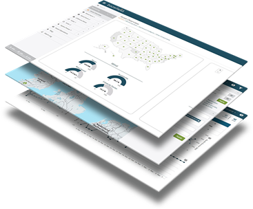
The power curve application contains 5 views: Graph, Data, Compare, Wind Rose and Energy rose

Figure 1 Power Curve Analyzer main chart view
3.1 SUPPORTED PLATFORMS
BazeField is designed using responsive design patterns, and supports a wide range of devices from mobile phones and tablets to desktop computers. The Power Curve application requires no client installation and supports most modern browsers like Chrome, Firefox, IE11 and Safari.
The power curve graph view contains 3 parts which is explained in the following chapters - Graph
4 USING THE POWER CURVE ANALYZER
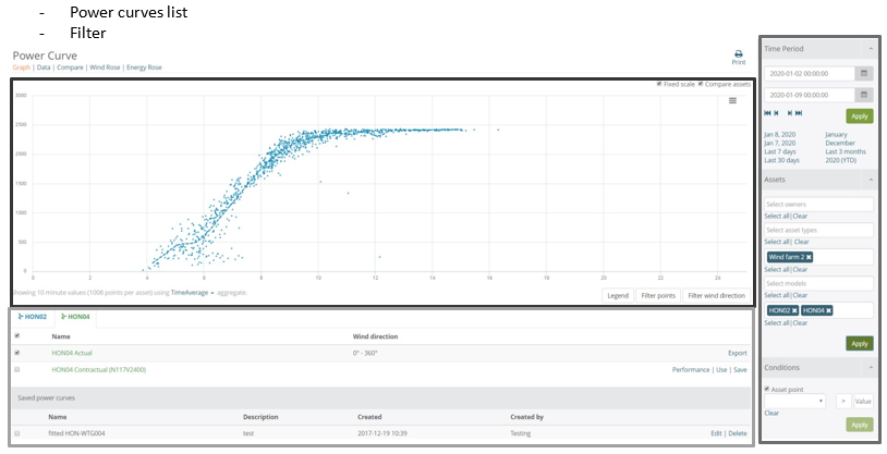
Figure 2 Power Curve Analyzer overview
To select asset, use the asset dropdown below the heading.
When the Compare assets checkbox is checked, up to 3 assets may be compared at once. See more about this in chapter Power Curve Analyzer with multiple 5.
4.1 GRAPH
The graph displays miscellaneous power curves, where the x-axis represents wind power (m/s), and the y-axis represents the active power produced by the asset (kW). By default, 3 power curves will be presented in the graph per selected asset:
- Actual (scatter) – The measured points that are returned from the DataEngine.
- Fitted – A power curve that is calculated from the Actual power curve.
- Contractual – The asset models contractual power curve, specified by the manufacturer.
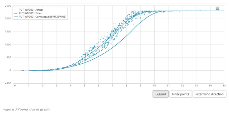
Power curves may be hidden or displayed by clicking on the names in the legend in the upper left corner. Power curves may also be added or removed from the chart completely by toggling checkboxes in the power curves list (see chapter 4.1.1). The visibility of the legend may be hidden by deselecting Legend button.
The chart may be exported to images in different formats, pdfs or svg vector images by clicking on the button in the upper right corner of the chart, as shown in the image below.

Figure 4 Exporting graphs
The Filter wind direction button is used for filtering the curves by selecting a desired wind direction range. This functionality is explained in chapter 6.
The Filter points button is used to remove outliers in the data set by drawing an area in the chart. The resulting fitted curve may then be saved for future reference and comparison. Read more about this in chapter 7.
4.1.1 POWER CURVES LIST
Power curves for the loaded asset(s) and previously saved curves are displayed in the lists. By toggling the checkboxes next to their names, the curves are added or removed from the chart. If a wind direction filter is applied, the selected wind range will be displayed in the wind direction column.

1 Power curves lists
4.1.1.1 EXPORT
The Actual power curves may be exported to a csv file by clicking the Export button. The csv file may then be analyzed further in other applications, for example Excel.
4.1.1.2 SAVE
The fitted and contractual power curves may be saved by clicking the Save link-button. The saved power curves will then appear in the saved power curves list, and may then be loaded into the graph at any time for comparison.
4.1.1.3 UNDER PERFORMANCE
Underperformance detection is useful for finding turbines that are underperforming compared to theoretical performance.
Underperformance is detected by the server side services and visualized in Asset Operations, Analysis application, and Alarm log.
The trigger for identifying an underperforming turbine is set up in the Power curve application under the Performance function in the list as shown in the picture below. The trigger is based on the difference between actual production and theoretical production using the active theoretical power curve (update the active power curve by clicking the Use button in the screen below).

4.1.1.3.1 CONFIGURATION SETTINGS FOR UNDERPERFORMANCE
Click on the Performance link in the Fitted or Contractual power curves in the list. This will bring up a configuration form, shown below.

Time detection period (hours)
How long the turbine is detected as underperforming before an alarm is created.
Change in performance (%)
This configuration set the difference in percent that is needed to trigger an underperforming alarm. The trigger is based on the difference between actual production and theoretical production using the active theoretical power curve.
Minimum detection power (kWh)
Minimum turbine power, where the underperformance watch should start.
Alarm description
The description of the alarm that will occur in the alarm log.
Distribute detection to all assets of same model
Use these conditions to distribute same trigger configuration to detect underperformance for all turbines of the same model.
For the configuration link to appear in the PowerCurve application an administrative setting,
UserPowerCurvePerformanceDetection, must be turned on in settings (see administrative settings) and also in BazeField.Services.AppSettings.config the key UnderPerformanceTagNamePattern must be set:
<add key="UnderperformanceTagNamePattern" value="%SITE%-%TURBINE%-PerformanceAlarm600"/>
Underperformance will show as alarms in Alarm Log like this:

Side-note: Could be extended to support other types of underperformance such as ice-detection, nacelle misalignment, as examples. For each new alarm-type a trigger-calculation must be set up. Each turbine vendor have different sets of tags available so these triggers must be configured on customers request.
4.2 THE FILTER
The Power Curve Analyzer uses the filter for selecting turbines and specifying the time period for the generated power curves.
The filter contains handy shortcuts for quick-selecting time periods.
When the filter is applied with any of the Apply buttons, the power curve(s) is generated.
If the Power Curve is in multiple turbines mode, the turbine filter is used to select the specified turbines. Read more about this in the chapter 5.
4.3 DATA VIEW
The data view lists the data set from the Actual power curves.
By clicking on the headers the list is sorted ascending. Click again, and the list is sorted descending.

An export function is available in the bottom of the list for each turbine, resulting in a comma separated values file.
4.4 COMPARE

4.5 WIND ROSE
The wind rose chart gives a succinct view of how wind speed and direction are distributed at the asset location. The directions of the rose with the longest spoke show the wind direction with the greatest frequency.

By selecting degrees the precision can be altered.
To view and compare individual assets show as induvial chart to view several assets summarized wind rose selected summarized chart.
![]() By clicking on the wind ranges in the legend below the wind rose, the graph will refresh accordingly, showing only the selected wind ranges. This is a nice tool for magnifying and analyzing the smaller areas of the chart.
By clicking on the wind ranges in the legend below the wind rose, the graph will refresh accordingly, showing only the selected wind ranges. This is a nice tool for magnifying and analyzing the smaller areas of the chart.
4.6 ENERGY ROSE
The Energy Rose chart gives a succinct view of how active power and direction are distributed at the asset location. The directions of the rose with the longest spoke show the highest active power.

To view and compare individual assets show as induvial chart to view several assets summarized wind rose selected summarized chart.
4.7 ADMINISTRATIVE SETTINGS
The administrative settings require administrative access. Here there are a set of settings that determins the behavior of the Power Curve application.
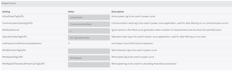
4.7.1 ACTIVEPOWERTAGSUFFIX
- Active Power tag to be used in power curve
4.7.2 COMMUNICATIONSTATETAGSUFFIX
- Communication state tag to be used in power curve application, used for data filtering on no communication errors
4.7.3 MINBUCKETCOUNT
- Ignore points in the fitted curve generation when number of measurements are less than the specified input
4.7.4 OPERATIONSTATETAGSUFFIX
- Operation state tag to be used in power curve application, used for data filtering on run state
4.7.5 USEPOWERCURVEPERFORMANCEDETECTION
- Use Power Curve Performance Detection
4.7.6 WINDDIRECTIONTAGSUFFIX
- Wind direction tag to be used in power curve
4.7.7 WINDSPEEDTAGSUFFIX
- Wind speed tag to be used in power curve
4.7.8 WINDSPEEDTHEORETICALPOWERCALCTAGSUFFIX
- Wind speed tag to be used for calculating theoretical production
5 POWER CURVE ANALYZER WITH MULTIPLE ASSETS
By checking the Compare Assets checkbox, up to 3 assets may be added for comparison purposes. Each added turbine is then represented by a unique color.
If 2 or 3 turbines are already selected in the filter, these will automatically be applied. If more than 3 turbines are selected, the filter will be applied with the current turbine, and a message box will appear:


3. Comparing power curves
Turn on and off the power curves by clicking on the legend or remove and add curves by checking the boxes in the list below the chart.
The scatter- and wind direction filter is also available in multiple assets mode. When used, these functions will then be applied to all the active turbines.
![]() There is a limit of 3 assets that may be loaded into the chart at once. This limit is set because of performance. A warning will appear when selecting more than 3 assets in the filter and the 3 first assets will be displayed.
There is a limit of 3 assets that may be loaded into the chart at once. This limit is set because of performance. A warning will appear when selecting more than 3 assets in the filter and the 3 first assets will be displayed.
6 POWER CURVE ANALYZER WITH WIND DIRECTION FILTER
The Power curve analyzer includes a wind-direction filter that enables visualization of power curves filtered by any windrange.

When pressing the Filter wind direction button in the bottom right of the chart area, a wind-direction widget will appear.
 The wind direction range is set by dragging the wheel, and the start degree is set by using the buttons beneath. [<<] skips 10 degrees backwards, [<] 1 degree backwards, [> 1] degree forward and [>>] will skip 10 degrees forward. When holding the buttons down the range moves accordingly.
When the desired wind range is selected, hit Apply, and the new filtered measurements and new fitted curve will be displayed. A read-only wind-direction widget will then also be displayed in the graph to indicate that the curves are filtered.
![]() When changing assets or reloading data sets, the wind direction filter will be cleared.
When changing assets or reloading data sets, the wind direction filter will be cleared.
7 POWER CURVE ANALYZER WITH MANUAL OUTLIER REMOVAL
The application includes a genial manual data validation /eraser function for quick and intuitive removal of outliers in the data set. Then fitted power curves can be calculated with very high precision and then be used for calculation of for more accurate power forecast / theoretical production.
The outliner removal tool is accessed by clicking the Filter points button. The chart will then go into filter mode. Then, by drawing with the mouse pointer in the plot, the scatter points in the drawn areas are marked for removal. The manual data validation / eraser are shown below:

4 Filtering scatter points
By pressing Apply, new Actual and Fitted curves are redrawn. The figure below shows the result after the scatter removal. The resulting fitted curve may then be saved for future references, and will appear in the saved power curves list.

5. Filtered scatter
The filtered data sets may at any time be reverted to the original result by pressing the Clear button.
The outlier removal tool may also be used when comparing turbines. Scatter points marked for removal from all turbines will then be removed at once.
8 LIMITATIONS
By default the Power Curve Analyzer displays 10 minutes average values from the turbine. To avoid slow performance 1.000 scatter points are loaded per graph as default. If the chosen time-period exceeds 1000 points for a turbine, the sample interval is increased. When this happens, a message will appear displaying the new sample interval and a function to override the 1.000 points per turbine limit:

Max scatter-points allowed for the graph in total is 10.000. If the requested number of points exceeds this number, a warning message will appear:
