
User Manual
Bazefield Availability
INNHOLDSFORTEGNELSE
3 INTRODUCTION
In order to improve availability, keeping track on all stops and alarms generated by the turbine control system it is essential to thoroughly investigate and understand the root error cause(s) and take actions on stop events.
BazeField 6 now provides a brand new application called Availability which replaces the older Stop Analyser and Loss Analyser applications. The new Availability application has many new and enhanced features and enables the user to manage availability in a powerful and user-friendly way.
The application also shows the availability for each asset in the time line, and calculates both asset availability and data availability for a selected period.
The application supports multiple availability calculations and categorizations views. Both IEC 61400-25 (time based) and IEC 61400-26 (production based) is included by default, but other classifications can easily be configured. This can be contractual, ISP contractual, technical categorizations according to IEC 61400 or RDS-PP etc.
The application also has a separate statics page with bar, pie and waterfall visualizations.
3.1 SUPPORTED PLATFORMS
The Availability application requires no client installation and supports most modern browsers like Chrome, Firefox and IE11.
4 ALLOCATIONS
When starting the application the “Allocation” view opens and displays the timeline for all assets selected in the filter. Each allocation represents a time period which has a certain category (i.e Timebased IEC 61400). The application also shows the total allocation found for the specified time interval and the number of assets.
 NB! If a smaller time period than “Day” is selected in the filter then the application will still display a timeline for a whole day. The time period is always rounded up to the nearest whole day.
 Figure 1. Allocations
4.1 AVAILABILITY TYPES
The availability type can easily be changed by selecting another in the dropdown next to the application title.
4.2 TIMELINE
Allocations are shown on the timeline using colors relevant to each availability type. Allocations marked with a “black line”(  ) are manual override allocations that supersede an automatically generated allocation. When there are no allocations the timeline is displayed as green. Hold the mouse over an allocation in order to show a tooltip with the category and more detailed time information.
 Figure 2. Allocation override
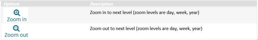
The timeline contains some tool buttons with the following options:
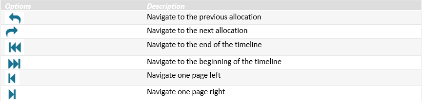
 NB! You can also use the scrollbar to navigate forward and backwards in time or use the finger for scrolling on tablets.
The application also contains a top level toolbar with the following options.
4.2.1 ADD BULK EVENT
It is possible to add a bulk event that will affect all selected assets in the filter in the given time period.
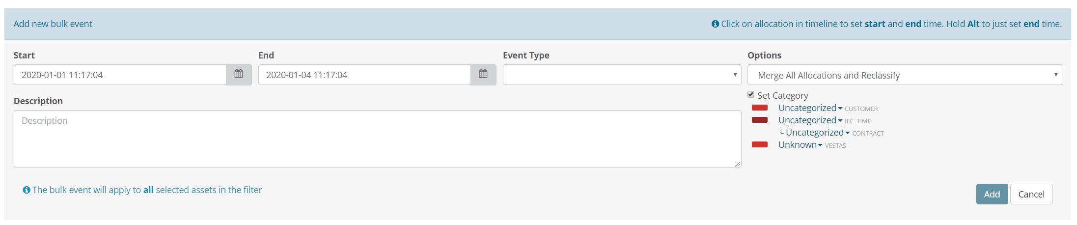
It is possible to either use the start/end datetime pickers or use the mouse.
To use the mouse click on allocation in timeline to set start and end time. Hold Alt to just set end time.
4.3 NAVIGATION
There are several ways of navigating using the allocation timeline.
- Click on an allocation to navigate to the Override view (see chapter 5). It will show the override view centered on the selected allocation.
- Click on the green timeline to navigate to the Override view (see chapter 5). It will show the override view centered on the clicked position.
- Clicking on just the Override view link will navigate to that view (see chapter 5). It will show the first turbine in the list and retain the same scroll position.
4.4 ALLOCATIONS
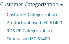
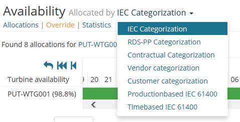
By default the system is configured with two different allocation categorizations, Timebased IEC and Contractual Categorization. However, the number of categorizations is dynamic and based on the alarm configuration file imported for each turbine type individually. Visualization of allocations in the application such as colors and categorization names are also configurable. The picture below shows an example of some categorizations.
5 ALLOCATION OVERRIDE
 Figure 3. Allocation override
5.1 OVERRIDE
To override an allocation, find the appropriate allocation and click the Override link.
 Figure 4. Original allocation before override is clicked
A new allocation is then created which overrides the existing allocation. The overridden allocation is shown with a black line indicating that this allocation is created manually.
 Figure 5. Overridden and original allocation after override is clicked
Click the edit button to change categorization or start and stop time for the allocation.
There is also a function available to display both the overridden allocations and the original allocations at the same time.

5.2 SPLIT
Each allocation can be split in two or more allocations. An individual root cause and categorization can be set for each new allocation split from the original allocation.
The original allocation will always be present in the database, however it will be presented as Overridden in the list. The statistics created will also neglect the registration and use the split registrations instead.
5.3 MERGE
Two or more allocations can be merged together as one. The statistics will make use of the merged allocation when statistics are calculated.
5.4 DELETE
Delete functionality can only be used on added allocations such as: split, overridden and merged. Simply mark the allocation in the allocation list and click delete to permanently remove the allocation chosen.
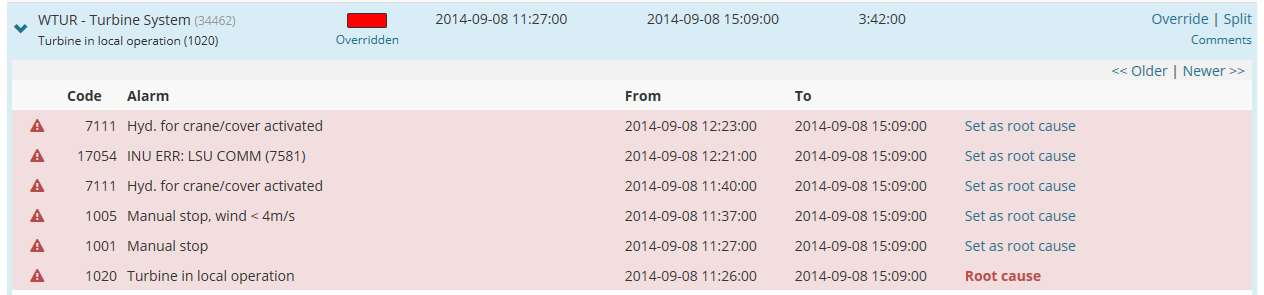
5.5 ROOT CAUSE
In some situations there is a need to change the root cause of an allocation to improve statistics. To change the root cause, open the alarm list related to the allocation by clicking the > icon to the left in the allocation list as shown in the table list below. Each alarm that is related to the allocation (between the start and stop time) are presented in the list with a light red background color.
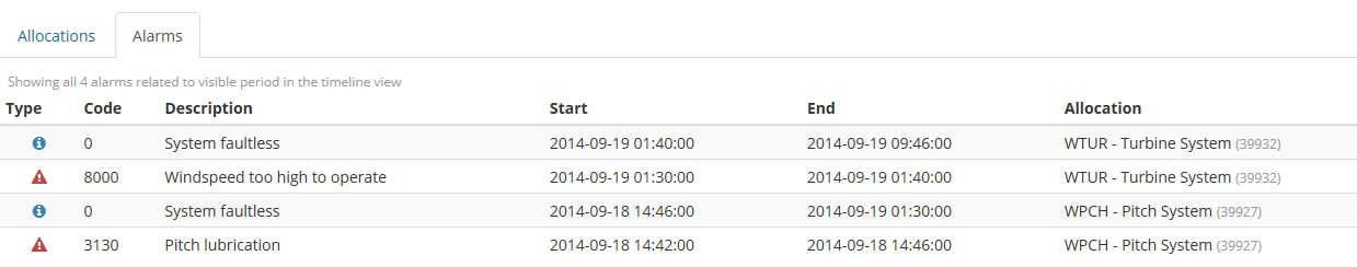
5.6 ALARMS
All alarms related to the chosen turbine for a given site during a filtered period are presented in an alarm list that appears as you click on the Alarms tab folder in the application. An example alarm list is shown in the screen below.
6 STATISTICS
The statistics page offers a convenient overview on what stop allocations that are most common. It includes graphs for the top 10 allocation categorizations distribution, KPIs, and a more detailed list of the visual presentation. Full Performance is not included as this is a run category.
6.1 TOP 10 ALLOCATIONS GRAPH
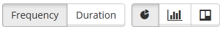
The top 10 allocations graph displays the 10 most common allocations in a pie chart, bar chart, or waterfall chart. The chart type is selected by these buttons.
By default the report displays the most common allocations by how many times they appeared (frequency). By switching to duration, the report shows the ratio between the length of the overall time of the allocations.

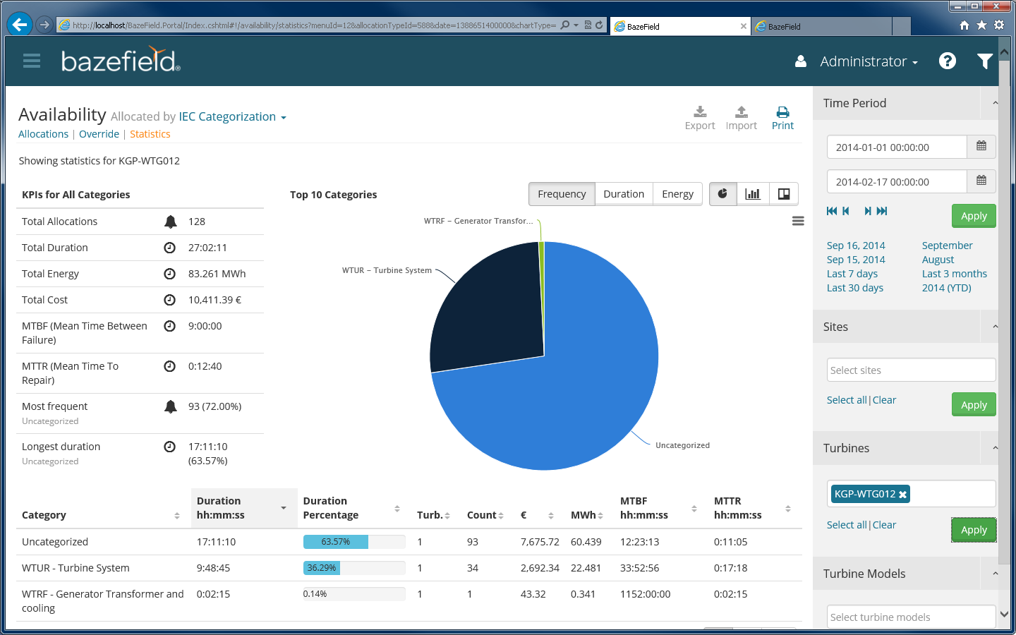
Figure 6 Statistics
The chart may be exported to images in different formats, pdfs, or svg vector images by clicking on the button in the upper right corner of the chart, as shown in the image below.
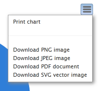
Figure 7 Exporting graphs
6.2 KEY PERFORMANCE INDICATORS
By default the KPIs shows information for all the allocations returned in the selected parameters with the filter. In the example below, the KPI area shows allocations for a turbine in a one month period.
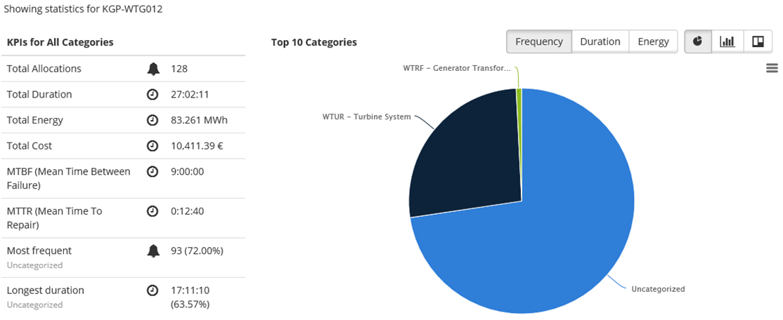
Figure 8 KPIs for all allocations selected by the filter
By clicking on a pie in the chart, the KPIs changes to only display KPIs for that specific allocation message. A blue information box also appears to make the user aware of this. Click once again on the selected pie or the provided link in the message to display the KPIs for all allocations.
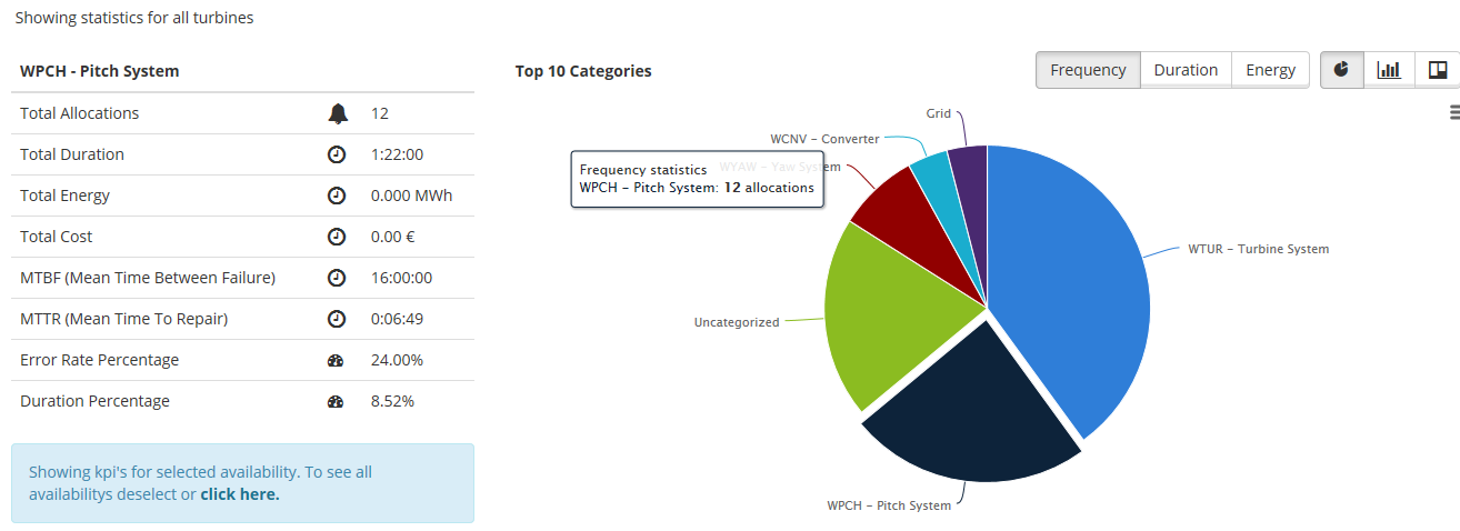
Figure 9 KPIs for a specific allocation message selected in the chart
6.3 ALLOCATION STATISTICS TABLE
For the chosen site, turbine(s), and time period the allocation statistics are calculated and displayed in a table list as shown in the screen below. If the system is configured with theoretical power curves and price information, then the system will display statistics on lost production and lost money as shown in the table below.
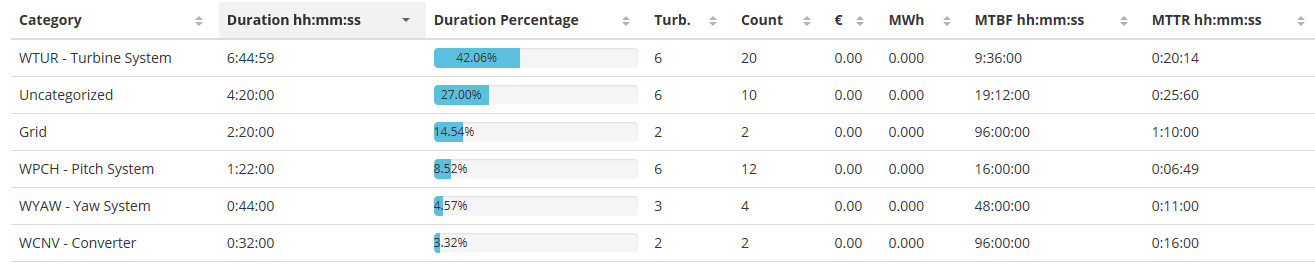
Figure 10 Allocation statistics table
In the table above, the figures in the MWh column are calculated based on the theoretical power in the period when the turbine was in a stop condition.
The lost revenue column named as: €, £, $, SEK, or some other local currency, is calculated based on the lost production in the period multiplied with the given price of electricity. By default the price information is retrieved from the Nordpool market price on an hourly basis. In some deliveries the price information also includes green certificate prices.
MTBF – Mean Time Between Failures. This is calculated as the total time period divided on the number of occurrences in the period.
MTTR – Mean Time To Repair. This is calculated as the total duration of downtime divided on the total number of stops within the given category.
6.4 DETAILS
The details list shows all allocations with the same KPIs as when selecting a pie in the chart.